Radar Altimetry Waveform Calculations Using
3D Raytracing And Precision Terrain Databases |
|
|
Here I discuss the application of my raytrace codes for modeling the temporal waveforms from radar altimetry instrumentation over rough terrains.
Currently, several very precise radar altimeters are being flown on satellites to measure the heights of the oceans on a continual basis. The form of the return signal reflected from the oceans is usually fit to a simple mathematical expression whose parameters are directly related to the oceans' levels. Now, there is interest to extend the mission of these altimeters to measure the heights of fresh water bodies over land, viz. large rivers and lakes. However, the character of these reflected signals differs markedly from those of the relatively flat oceans, and no simple mathematical function can be fit to these data. The signal returned from these flat water bodies is corrupted by the return from the much rougher terrain composed of vegetation, hills, buildings, roads, etc. It's not clear how to extract the heights of just the water bodies in these situations.
As part of an effort to develop the mathematical techniques to extract over-land water heights using radar altimetry, I've developed a technique to calculate the waveform returned from a known 3D terrain description. This technique uses raytracing with a lidar derived terrain database which characterizes an area by its constituents: land, vegetation, and roads. The advantages to this approach are several: 1) the return signal from the constituents can be isolated and compared for importance, 2) the corrupting effects of multipath reflection can be analyzed for influence, and 3) the results from all new algorithm development can be compared against the terrain database as truth.
Below, I describe the terrain used for this demonstration, show some interesting multipath raytrace phenomenology, and present my calculated waveform with discussion.
|
|
|
|
3D Terrain Description
|
|
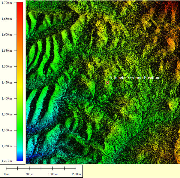
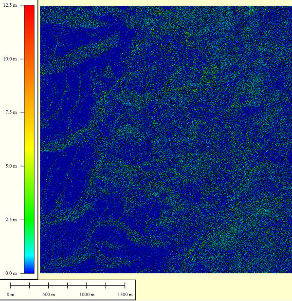
The 3D terrain data, vegetation, and road layers used for my demonstration calculation are shown in this panel. These databases were derived from lidar instrumentation flown over this region. The lateral sample spacing is 0.5m/pixel. The terrain dimensions were limited to 3.3Km by 3.5Km, or 6601 by 7001 samples, as dictated by the capabilities of my home computer. (The interesting 25Km by 25Km extent awaits analysis after acquisition of a workstation class computer.) Lidar terrain digitizing technology also identifies database constituents, which is important to altimetry modeling since each material type will reflect radar rays differently. The composition of the 46,213,601 samples breaks down as: 22,935,315 ground pixels, 23,103,563 vegetation pixels, and 174,724 road pixels. No buildings are present at this locale.
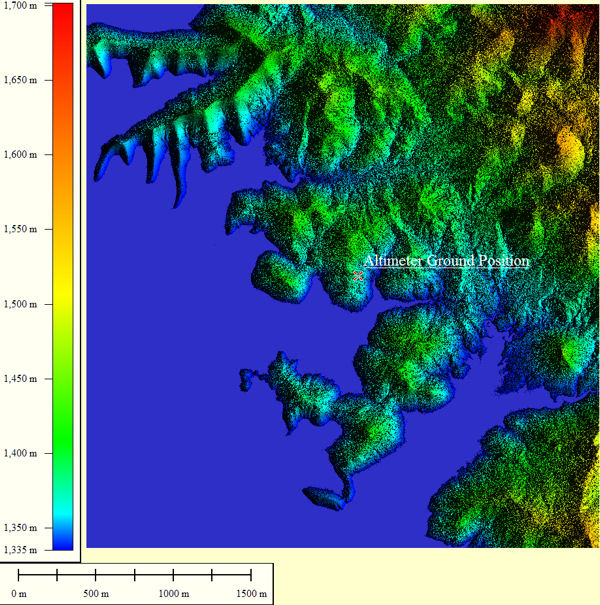
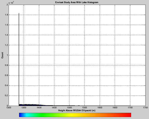
And there are no large water bodies in this example either. However, for future studies, a large body of water can be added to this database, as shown at the bottom of this panel. This high precision, waterless terrain was selected because it's availability coincided with a set of actual altimeter waveforms acquired at this position. The good comparison of my calculations to the actual waveforms is not discussed here.
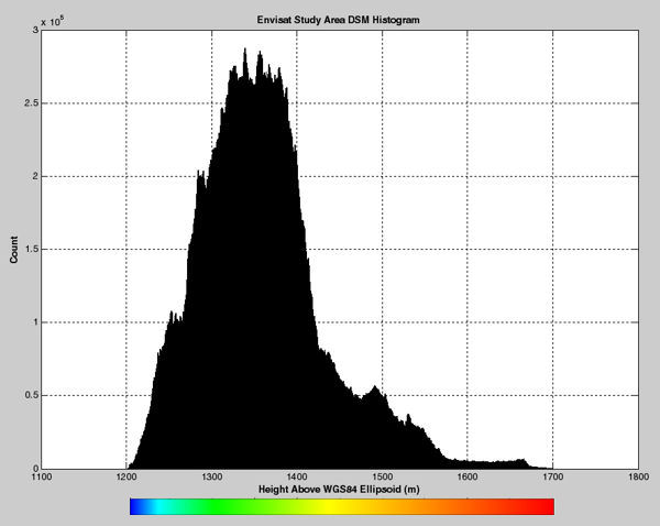
As a side note to the terrain histogram, if all rays hitting the ground perfectly reflected back to the altimeter with the same amplitudes, the derived waveform should correspond to this histogram--but with the abscissa reversed. In practice, the impinging rays reflect with differing amplitudes and different distances due to multipath propagation effects. An example of this is shown in the next panel.
|
|
Overhead View Of Terrain Study Area; 3.3Km by 3.5km
|
Terrain Height Histogram
|
|
|
Overhead View Of Study Area Vegetation Layer
|
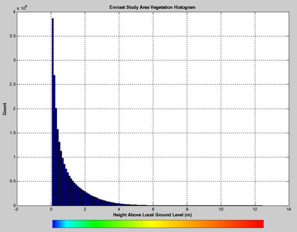
Vegetation Height Distribution With Respect To Ground
|
|
|
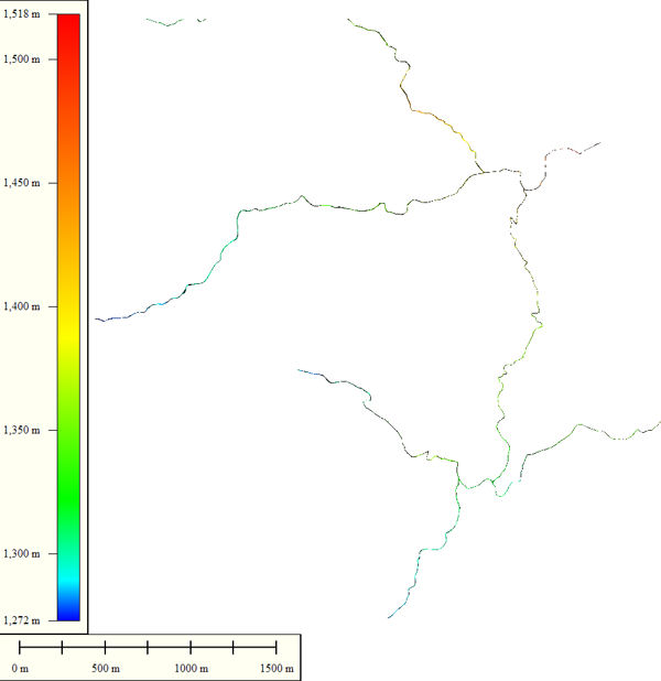
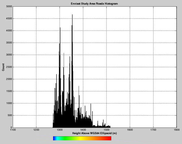
Roads Run Through This Terrain
|
Envisat Study Area Roads Histogram
|
|
|
Envisat Study Area With 'Lake Dennis'
|
Envisat Study Area With 'Lake Dennis' Histogram
|
|
|
|
Some Raytrace Examples
|
|
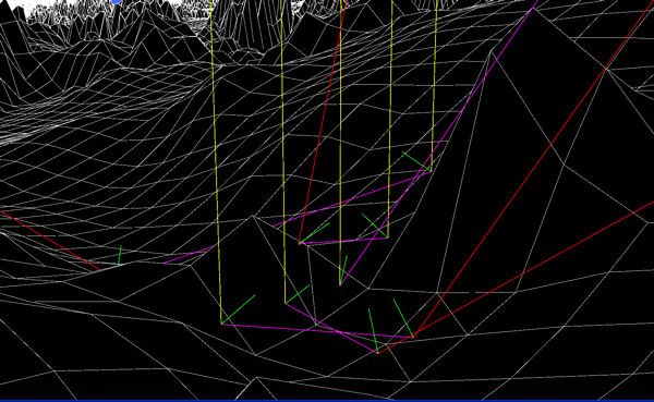
The two examples in this panel have been selected to highlight multipath ray propagation in our triangle-tessellated terrain.
The first picture on the left is a closeup showing five input rays (yellow) propagating down from the altimeter and reflecting off the terrain. Four of these rays reflect twice while the middle reflected ray propagates to infinity. The magenta lines are the first reflected rays; the red lines are the second reflected rays; the green lines are the facet normals at the points of reflection. My software propagates rays from the altimeter to all 6600 by 7000 polygons and tracks points of intersections and material bounce type for up to two bounces per input ray. I've written what I call a dual-resolution, supercover algorithm to calculate this efficiently.
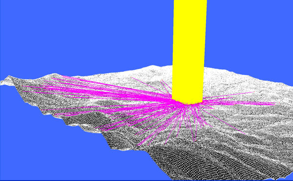
The second picture on the right shows an array of 500 by 500 input rays (yellow) from the altimeter striking the ground. (The rays are so dense at this resolution that they appear to be a plane.) And only the reflected rays (magenta) not going to infinity are plotted to emphasize that some reflected rays will appear to derive from a terrain height farther away than in actuality. The extent of this phenomenon over the entire terrain needs to be further analyzed.
|
|
MultiPath Propagation Rays: Yellow-Input, Magenta-First Bounce, Red-Second Bounce
|
500 By 500 Input Rays
|
|
|
|
Waveform Calculation Result
|
|
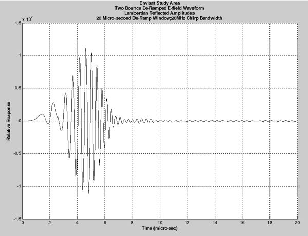
An altimeter can be viewed as an instrument that measures echo delay times and converts that information to distances. Following the design of a current satellite-borne altimeter, I've modeled the altimeter as a point source of (6600 x 7000) rays that interact with the terrain up to two bounces. The modeled altimeter therefore sees a returned electric field from each ground reflection point that has an amplitude and round trip travel distance. The instrument's front end electronics converts round trip travel time to round trip distance via the de-ramping process. In words, the de-ramped waveform is the sum of N sinusoids whose amplitudes depend on the individual ray's return strength and whose frequencies depend on when they appear in the de-ramp window. It is that waveform I have calculated and show in the left picture of this panel.
Further, for this calculation I've chosen a 20 micro-second acquisition window and a 20MHz chirp bandwidth. The satellite was located 798.629 Km above the ground position seen in the terrain overhead view shown above. The total round trip path difference between ray maximum and minimum propagation distances was 5141.25m, even though the terrain database itself only has a single-pass height difference of 498.149m. In the absence of real descriptions of material BRDFs, I (arbitrarily) chose to model the reflectors as Lambertian with relative amplitudes assigned as: roads(0.0db,) vegetation(-3.1db,) and ground(-10.1db.) My model can easily accept more accurate BRDF descriptions.
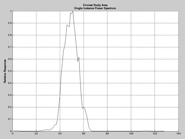
Finally, the picture of the power spectrum on the right was derived from the de-ramped waveform by first: applying a Hamming window to the data; second: performing an FFT; and lastly: squaring the result. This power spectrum should be compared to the terrain database histogram shown above. Only a single instance of the waveform was calculated and processed. Typically the radar altimetry community receives the average of 100 individual power spectra.
|
|
Calculated De-Ramped Electric Field Return Waveform
|
Power Spectrum of Calculated De-Ramped Waveform
|
|
|
|
|
Request More Information About Radar Altimetry Calculations
Author:Dennis M Hancock |
|
| View Dennis' Resume |
|
| Return To Dennis' Home Page |
|
|
| All Pictures on this Website Page are copyrighted by Dennis Hancock |
| ©2010 Dennis Hancock |