RADAR (AND OPTICAL AND ACOUSTIC) 3D RAY TRACING
WITH HIGH PRECISION LIDAR TERRAIN DATABASES
Recently, I've been writing and applying 3D ray trace codes to simulate ground, air, and space radar performance. This software models transceiver platforms at any height and any relative state of motion with respect to the target of interest. Both straight line and differential ray modes of propagation are modeled. The differential propagation mode is necessary for calculating beam bending in Earth's inhomogeneous atmosphere, which is typically of interest for ranges beyond 15km. These codes run on the latest parallel computer architectures and the outputs of this "virtual radar" are used for a variety of purposes, for example, estimation of standard Pd system metrics.
For certain classes of radar modeling, I've also developed a much faster algorithm (~ x5000) than ray tracing which lack ray bending and accurate optical path calculation.
Particular attention to execution efficiencies has been addressed by structuring software that capitilizes on knowledge of hardware architecture. Terrain database sizes equivalent to 8000 miles by 8000 miles sampled at 0.5m can be accommodated on a 32bit computer. Currently, terrain databases of very large size with high spatial resolution are acquired by lidar instrumentation.
Typical computed variables include:
- Target signal strength
- Scene clutter
- MultiPath
- Line of sight (LOS) visibility
- Line of sight invisibility (terrain masking)
- MultiPath Line of sight (MLOS) visibility
The types of phenomena that can be realistically modeled as Virtual Radar Signal Simulators:
- Satellite occultation
- Multipath exploitation radar
- Perimeter and border surveillance radar
- Propagation in inhomogeneous atmospheres
- Scintillation, ducting
- The Green Flash (dispersive, differential propagation)
- Wind turbine radar modeling
- Synthetic aperture radar (SAR) simulators
- Over the horizon radar (OTH) simulators
- Radar altimetry
Some application domains would include:
- Radar placement for maximum ground path surveillance coverage
- Calculation of shadowed areas invisible to ground radar placement (sometimes called terrain masking)
- Sniper placement
- Shadows cast (or removed) by proposed new buildings or vegetation
- Human gait analysis
I'm Available To Consult For Your Raytracing Project
Radar Visibility Model
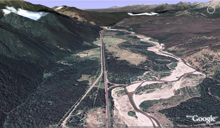
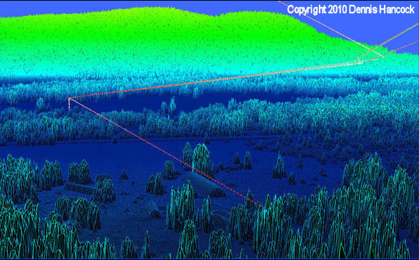
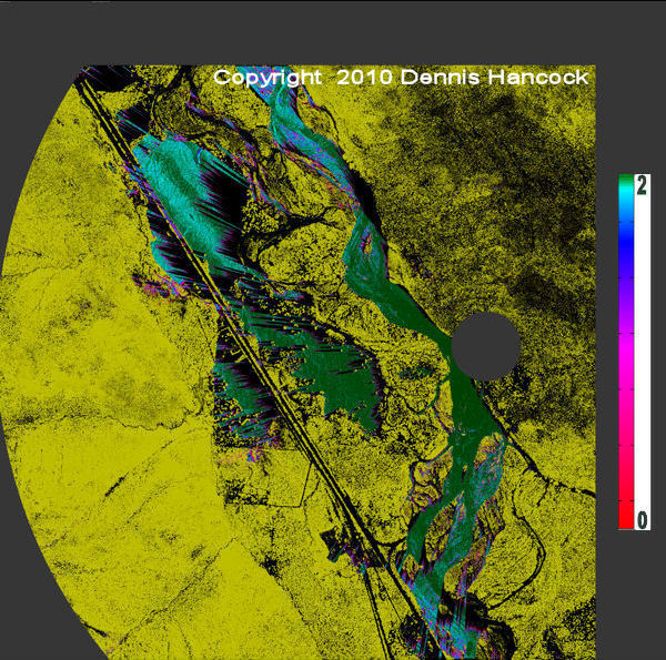
The following example using raytracing to calculate signal strength and clutter for a stationary ground radar pertains to a freely available, lidar-acquired terrain database for a forested, mountainous region 4.25 Km by 4.25km on a side. The lateral resolution for this geometry is 1.0m and the vegetation layer may be inferred at the same resolution. The differential mode was used to propagate the scene figure rays in an inhomogeneous atmosphere. Though these rays are slightly and continuously bending during propagation, the reason to do such is to estimate a more realistic optical path length. For K band radars, 50 waves of excess OPD can be realized over a 6Km range propagating horizontally to the ground. The signal strengh and clutter images are color coded for range-normalized electric field amplitude. (Note the tree shadows in the open field for this particular transmitter siting.) The colors not in the colorbar scale connote shadow (black) and vegetation (yellow.) It's important to point out that many places in the forest are seen by the radar; jpeg compression tends to mask those areas in these pixel-scaled pictures. Lastly, the radar placement for the signal pictures is different than the placement showing typical scene rays.
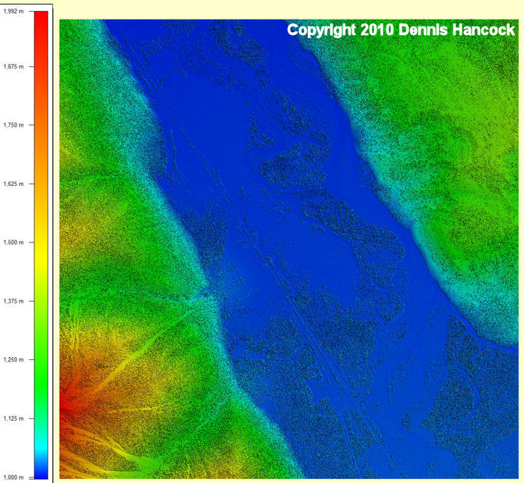 |
4.25Km by 4.25Km; 1m lateral sampling
 |
 |
 |
 |
 |
A note about the linear plotting scales for the pictures above. The Signal Strength is based on what height above the ground does the transmitter become visible. This is done on the basis of a 2.0m height. So for example, if the ground is directly visibile to the radar, that position is plotted green and has maximum signal strength. At the other extreme, if only the top of a 2.0m high person is visible, that position is color coded red and would have the least signal strength. Black connotes shadowing; yellow connotes vegetation which is ignored in these plots. The clutter signals are scaled to the cell with the largest amplitude. Assignment of engineering units would directly follow from knowledge of the transmitter power, beam pattern, and range.
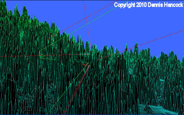
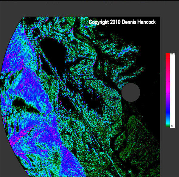
Clutter Movie
Radar signals returned from the same location in range and azimuth (cell) exhibit a variance in strength, particularly as the wavelength gets shorter (< 1 meter.) This behaviour, called speckle, is due to several factors effecting the plurality of scattered-waves' phases in each radar cell. The following movie displays calculations of the more difficult part of the radar return from the trees in this study area. The signal amplitudes are estimated as the coherent sum of all the scattering centers in the corresponding cell. In the absence of any other constraints, the scattered amplitudes are proportional to the exposed area of each tree in the cell; phases are randomly assigned a value over 2.0 pi on a frame by frame basis. The return from the ground is not modeled here, thus explaining the absence of signal (color coded black) from the visibile parts of the terrain. This type of simulation can be used to model the signal strength probability distribution function that is unique to a specific terrain and radar location.
 |
Scene Clutter From Forest
Author:Dennis M Hancock
Except the Google Earth view titled 'Satellite View Of Study Area'